
Methods
Biological Source Materials and Data Generation
Animal Culture and Collection
Oikopleura dioica were maintained in culture at 15°C as described (Bouquet et al., 2009). Oocytes were collected from mature females, and developmental stages up to and including metamorphosis were generated by in vitro fertilization (Schulmeister et al., 2007), with embryos left to develop in artificial sea water (Red Sea, final salinity 30.4-30.5 g/l) at room temperature to the desired stage. Day1-5 animals were placed in artificial seawater, chased from their houses, left for 30 min to empty their gut, anesthetized in cold ethyl 3-aminobenzoate methanesulfonate salt (MS-222, 0.125 mg/ml; Sigma), and then collected. Ovary and testes extracts were collected as previously described (Campsteijn et al., 2012). To obtain the trunk samples, Day5 animals were washed in cold phosphate-buffered saline (PBS) and anesthetized in cold MS-222, transferred to cold buffer A (10 mM Tris (pH 7.5), 360 mM sucrose, 75 mM NaCl, 10 mM ethylenediaminetetraacetic acid (EDTA), 10 mM ethyleneglycol bis[aminoethylether]-tetraacetic acid, 3 mM dithiothreitol, 1 mM phenylmethylsulfonyl fluoride, and 1:500 RNAse OUT (Invitrogen)) and gonads were punctured and removed. Remaining trunks were washed once in cold buffer A, pooled and processed for RNA isolation. For collection of the Day2-Day4 dense samples, the normal dilution of animal spawn at Day1 was omitted (Bouquet et al., 2009), yielding a culture with approximately 5-fold higher animal density. In partial compensation for elevated animal numbers while suppressing algal overgrowth, the food concentration was doubled at each developmental stage. The elevated animal density and feeding regime were maintained throughout the experiment, with animal collection performed at time points as indicated.
Developmental stages sampled
To assemble a complete developmental transcriptome for O. dioica, we subdivided organismal development into 12 segments. We began with unfertilized oocytes (‘Oocyte’) that are arrested in Metaphase I of meiosis. Oocytes were collected from females that were allowed to spawn naturally by rupture of the gonad wall. The next stage consisted of 2-8 cell embryos that encompass the maternal to zygotic transition in the transcriptional regulatory control of development. This was followed by a sample at 1h post fertilization (PF), a stage at which blastomere fates for most tissue types have already been determined (Stach et al., 2008). Continued rapid cell proliferation within determined blastomere lineages was captured by the ‘tailbud’ and ‘hatched’ stages, the latter stage occurring when the animal emerges from the protective chorion. The ‘early tadpole’ stage is a period of very active organogenesis. The ‘tailshift’ stage represents the completion of metamorphosis and initiation of filter-feeding. This was then followed by more spaced samples during which the bulk of animal somatic growth takes place (‘Day1’, ‘Day2’ and ‘Day3’). From the fourth day of development onwards, nutritional resources are increasingly allocated to growth and differentiation of the male and female reproductive organs (‘Day4’ and ‘Day5’). To specifically interrogate development of the reproductive organs, we collected samples derived from dissected and isolated testes or ovaries of Day5.5 animals, as well as a complementary animal sample consisting of Day5.5 animals with their gonads removed (‘trunk’). Importantly, we observed that culturing O. dioica at higher animal density (“restrictive conditions”) causes it to cease development and somatic growth just prior to germline differentiation at Day3 (Ganot et al., 2002). Therefore, we included three time points covering the entry into this developmental arrest (‘Day2 dense’, ‘Day3 dense’ and ‘Day4 dense’). Material derived from these 18 samples was processed and hybridized to tiling arrays.
Gene Annotation
A very detailed reporting of gene annotation protocols is provided in the supplementary information of Denoued et al., (2010). A summary version is presented here. SNAP ab initio gene prediction (Korf, 2004) was used to create a clean set of Oikopleura dioica genes. This set was used to train gene prediction algorithms and optimize their parameters. SNAP was launched using the Caenorhabditis elegans configuration file, and only models with all introns confirmed by at least one O. dioica cDNA were retained. Models that contained at least one exon that overlapped a cDNA intron were rejected. Three hundred models were randomly selected to create the O. dioica clean training set.
Exofish (Roest Crollius et al., 2000) comparisons were done with Biofacet. When ecores (Evolutionarily COnserved REgions) were contiguous in the two genomes, they were included in the same ecotig (contig of ecores). Exofish comparisons were performed between O. dioica and four organisms: Tetraodon nigroviridis, Strongulocentrus purpuratus, Ciona savignyi and Ciona intestinalis. High scoring segment pairs were filtered by length and percent identity.
The Uniprot (Uniprot Consortium, 2012) database was then used to detect genes conserved between O. dioica and other species. Since Genewise (Birney et al., 2004) is computationally intensive, sequences in the Uniprot database were first aligned with the O. dioica genome assembly using BLAT (Kent, 2002). Each significant match was chosen for a GeneWise alignment. The default GeneWise gene parameter file was modified to account for unusual splice sites of O. dioica genes. Geneid (Parra et al., 2000) and SNAP ab initio gene prediction software were then trained on the 300 genes from the training set.
Three full-length-enriched cDNA libraries were prepared from a cultured outbred population (large pools of unfertilized eggs, embryos at mixed stages from 1 to 3 h pf, tadpoles 6-10 h pf and Day 4 animals) and 180,000 cDNA clones were successfully end-sequenced. After assembly of 5’ and 3’ sequences, a total of 177,439 sequences were aligned to the O. dioica genome using the following pipeline: after masking of polyA tails and spliced leaders, the sequences were aligned with BLAT on the genome assembly and matches with scores within 99% of the best score were extended by 5 kb on each end, and realigned with the cDNA clones using Exonerate (Slater and Birney, 2005), allowing for non canonical splice sites, with the following parameters; --model est2genome --minintron 25 --maxintron 15000 --gapextend -8 --dnahspdropoff 12 --intronpenalty -23.
An NCBI (Sayers et al., 2012) collection of ~1,500,000 public tunicate ESTs was then aligned with the O. dioica genome assembly using BLAT alignments refined with Est2Genome (Mott, 1997). Significant matches were chosen for alignment with Est2genome. BLAT alignments used default parameters between translated genomic and translated ESTs.
The above resources were combined to automatically build O. dioica gene models using GAZE (Howe et al., 2002). Individual predictions from each program (Geneid, SNAP, Exofish, GeneWise, Est2genome and Exonerate) were broken into segments (coding, intron, intergenic) and signals (start codon, stop codon, splice acceptor, splice donor, transcript start, transcript stop). Exons predicted by ab initio software, Exofish, GeneWise, Est2genome and Exonerate were used as coding segments. Introns predicted by GeneWise and Exonerate were used as intron segments. Intergenic segments were created from the span of each mRNA, with a negative score (forcing GAZE not to split genes). Predicted repeats were used as intron and intergenic segments, to avoid prediction of protein coding genes in such regions.
The whole genome was scanned to find signals (splice sites, start and stop codons). In order to annotate genes containing non-canonical splice sites, all G* (GT, GA, GC and GG) donor sites were authorized. Segments predicting exon boundaries were used by GAZE only if GAZE chose the same boundaries. Each segment or signal from a given program was accorded a value reflecting our confidence in the data, and these values were used as scores for the arcs of GAZE automaton. All signals were assessed a fixed score, but segment scores were context sensitive: coding segment scores were linked to the percentage identity (%ID) of the alignment; intronic segment scores were linked to the %ID of the flanking exons. A weight was assigned to each resource to further reflect reliability and accuracy in predicting gene models. This weight acted as a multiplier for the score of each information source, before processing by GAZE. When applied to the entire assembled sequence, GAZE predicted 17,113 gene models on the reference assembly. The final proteome of 18,020 gene models was obtained by adding 907 gene models from an allelic assembly that were not present in the reference assembly.
RNA isolation, cDNA synthesis and quantitative RT-PCR
RNA isolation was performed using RNeasy (Qiagen) and RNA quality was assessed using a Bioanalyzer (Agilent). Purified total RNA was briefly treated (15 min at room temperature) with 0.5 units of DNase I (AMP grade; Invitrogen) per µg of RNA to remove residual DNA, followed by ethanol precipitation and purification of RNA. Double stranded cDNA was synthesized using SuperScript™ Double-Stranded cDNA Synthesis Kit (Invitrogen) according to NimbleGen protocols, followed by phenol:chloroform:isoamylalcohol (25:24:1), chloroform:isoamylalcohol (24:1) backextraction and ds cDNA was recovered by ethanol precipitation. Typically, 4-10 µg of input total RNA yielded 3-9 µg of ds cDNA. First strand cDNA synthesis and quantitative RT-PCR were performed as previously described (Campsteijn et al., 2012), and primer pair specificities were evaluated by melting curve assessment and amplicon sequencing. All transcript levels were normalized to RPL23 and EF-1-beta.
Tiling array hybridization and processing
A tiled genomic microarray was designed to interrogate the entire non-repeat genome of Oikopleura dioica based on genome sequence assembled in collaboration between the Sars International Centre for Marine Molecular Biology and Genoscope. For each developmental time point (or stressor), cDNA was labelled and amplified using the Roche NimbleGen gene expression protocol with the following modifications: 15 μg of the labelled cDNA was hybridized to each array, and hybridization was performed on 3 separate arrays (3 technical replicates). The arrays were washed and processed as per the manufacturer's recommendations, and the arrays were scanned on a Molecular Devices GenePix Axon 4400A at 5 µM resolution. The scanned array data were converted into pair and gff files, which were processed as indicated below.
Data Processing
Pre-processing tiling array data
Probe intensities across all technical replicates (4 for the oocyte sample and 3 for all others) were first quantile normalised. A smoothing function was then implemented across all non-random probes in each sample. A three-probe sliding window was used, across each scaffold, together with a calculation of the Hodges-Lehmann estimator of location (“pseudo-median”) across all replicate probes in the window (i.e. the pseudo-median of 12 probes in the oocyte sample and 9 in all others). This collapses the replicate probe intensities into one smoothened set per sample.
A background subtraction was then implemented using random probes. Random probes from all replicates for each sample were combined and ranked by intensity. A percentile cutoff of 2 was then chosen, after comparison to qPCR data (see below), representing a false positive rate of 2%. The intensity at this cutoff was used as a background threshold. The background threshold calculated for each sample was then subtracted from all non-random probe intensities and any resulting negative values replaced with zeros.
Since intron sizes in the Oikopleura genome peak at 47bp (Denoued et al., 2010) and the median probe length on the tiling array is 53bp an intron may be represented by a single probe, which would have been eliminated during the data-smoothing step. We therefore applied an additional step to recover these single probe introns. We carried out the background subtraction step as above on all normalised pre-smoothened non-random replicate probe intensities. For each probe we then calculated its median intensity across all replicates. If this median value was negative and its smoothened value was positive, we replaced this positive value with zero to recover the short intron this probe likely represented. Figure1 summarizes these pre-processing steps.
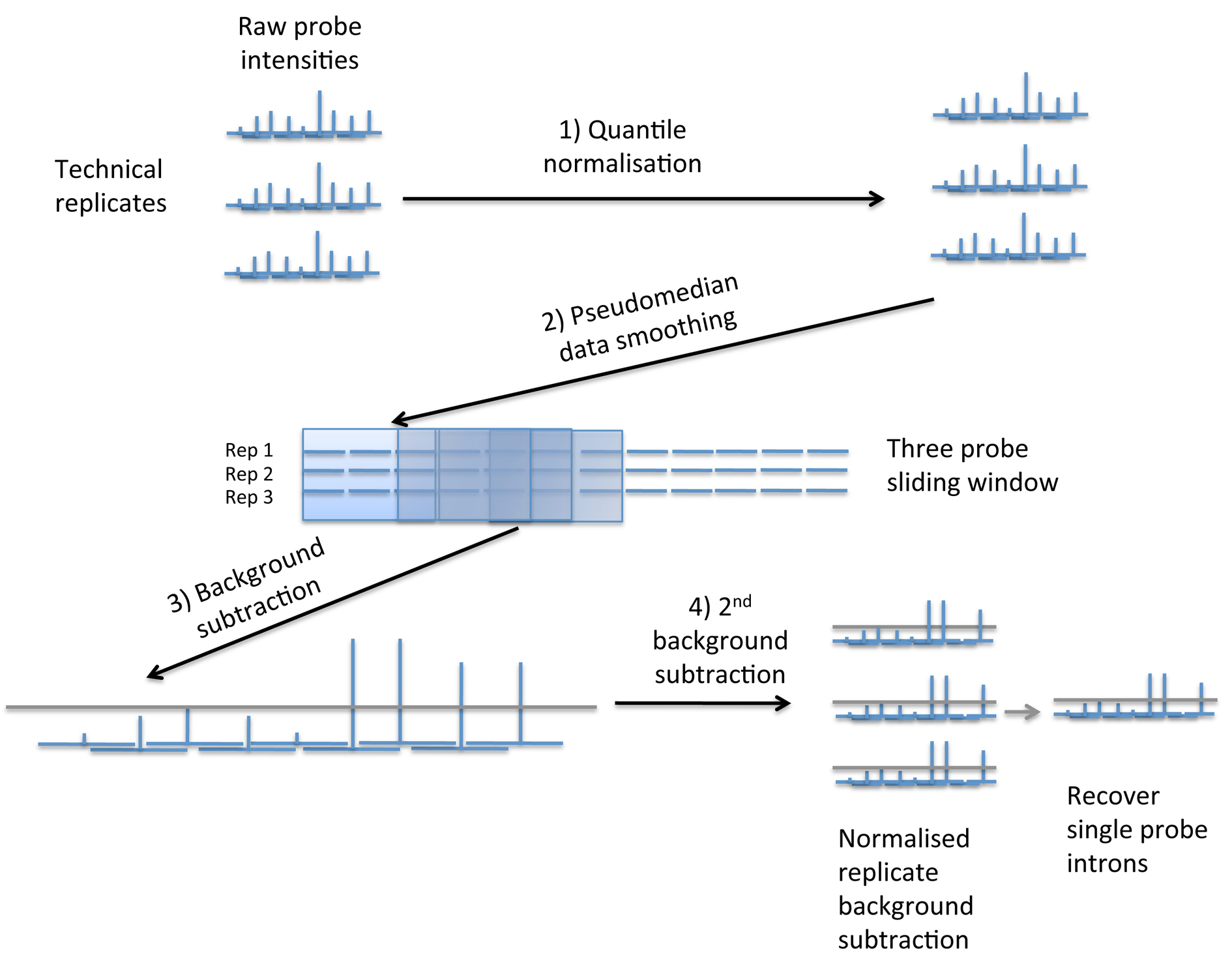
Figure 1. Pre-processing the raw microarray probe intensities in 4 main stages: 1) Quantile normalization between technical replicates for each sample individually; 2) using a 3-probe sliding window and the Hodges-Lehmann estimator of location (“pseudomedian”) to smooth the data and collapse the replicates; 3) background subtraction using the 2-percentile random probe value for each sample; 4) A second background subtraction step on all replicates individually to retrieve single probe introns (see text).
As a final step before further analyses we excluded probes that have the highest potential for cross-hybridization by removing any probes that occur more than 3 times in the genome as well as those that are within repeat regions as annotated by RepeatMasker and/or RepeatScout (Denoued et al., 2010), after merging these regions. This gave a total of 13.2% of probes excluded from further analyses.
Defining transcriptionally active regions (TARs)
We define a transcriptionally active region (TAR) as any stretch of consecutive positive probes in a particular sample. Given the presence of short introns in the Oikopleura genome, we allow single probes to separate TARs, and also allow short exons by allowing any number of probes to define a TAR. To compare TARs between samples we constructed a set of ‘superTARs’ that represent maximal continuous regions in which transcription occurs in any one or more samples.
Calculating gene expression
We used the set of Oikopleura gene models on the reference genome (Denoued et al., 2010) in calculating expression levels for each based on its annotated coding region. We assigned probes to annotated CDS regions of gene models where there was an overlap of at least 30 bp between them. For each gene model we then calculated an expression level in each sample by taking the median of all positive probes in that sample. We also calculated the proportion of probes that are positive for each CDS region and each gene model as a whole. We used this information to define three confidence classes for the expression level of each gene in each sample, where the gene expression is greater than zero. Any gene that has ≥50% of CDS probes expressed we define as being ‘high confidence’. Genes that have fewer expressed probes we then reassessed using a ‘two exon rule’: if two or more contiguous CDS regions have ≥50% of probes expressed we call this gene as expressed with ‘medium confidence’. For any gene that fails this rule we give it an expression level of zero in that sample. If the gene nonetheless has any one CDS region with ≥70% of probes expressed we define it as being a ‘low confidence’ gene, but assume that it represents cross-hybridization and do not consider it as expressed in downstream analyses. Figure 1 summarizes the processing of probe intensities to give gene expression levels along with their confidence categories.
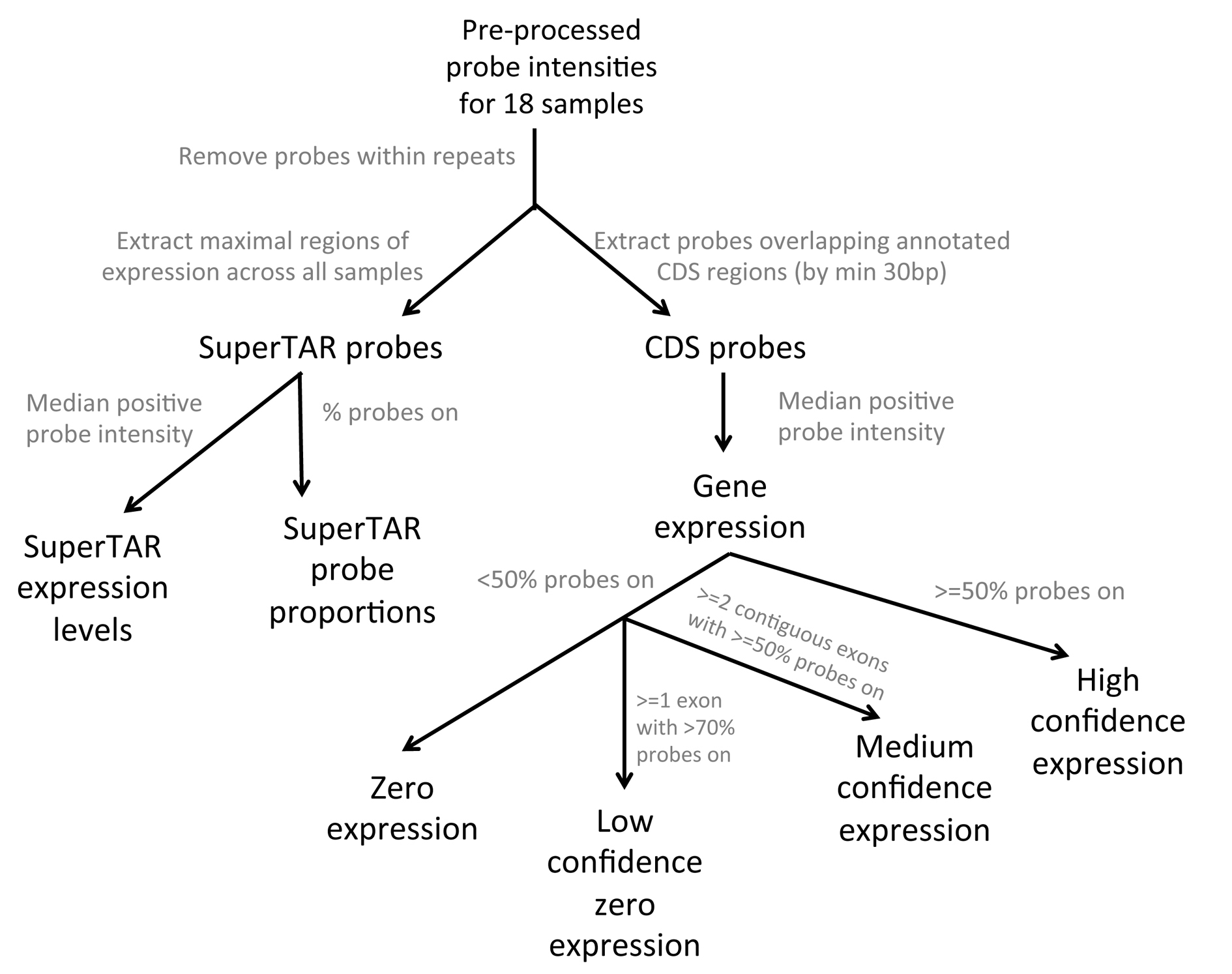
Figure 2. Processing the probe intensities in order to calculate gene and superTAR expression levels. Gene expression levels were further categorized for each sample based on the proportion of positive probes across the coding region.
Calculating superTAR expression
We calculated the expression levels of superTARs in unannotated ‘intergenic’ regions by taking a median of all positive probes within each superTAR for each sample. We also calculated the proportion of positive probes within each superTAR to use in assessing whether or not a superTAR is active in any one sample.
Validation and Assessment
Validating gene expression profiles and choice of parameters
We tested three different background thresholds in the pre-processing step using 1%, 2% and 3% of random probe intensities. We compared the expression profiles of 17 genes that have ‘high confidence’ expression levels in all samples against qPCR expression profiles in 11 (strictly normal development) out of 18 equivalent samples taken from both the same populations as used for the tiling array as well as independent populations. Overall the correlation between profiles using different thresholds was very high (Pearson’s correlation coefficient >0.96 in 16/17 genes). Where there were differences these tended to favour a 2% FPR (which had the highest number of highest correlation coefficients) and so we chose this to define a background threshold for each sample.
We also tested three different parameters for our ‘two exon rule’ used in reassessing the expression levels of genes with <50% of probes expressed. We allowed genes to be called as expressed if two contiguous CDS regions contained at least 50%, 60% or 70% of probes expressed. We then compared the expression profiles of a subset of 57 genes to their expression profiles using qPCR. Out of these only 8 genes were affected by the differing thresholds of the two exon rule and in most cases this favoured using a lower threshold. For example, one gene, cyclinB3b was only called as expressed on the array at a threshold of 50%. We therefore used this threshold in our two-exon rule.
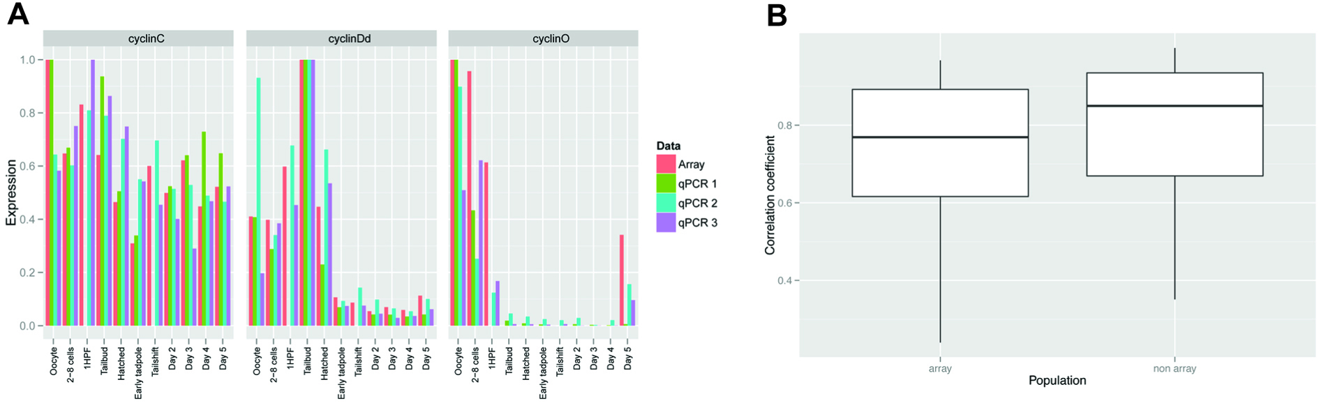
Using a 2% FPR in our background subtraction pre-processing step and a 50% threshold in our two-exon rule we compared the tiling array expression profiles to our set of 57 qPCR expression profiles in order to validate our approach (Figure 3 and Table 1). Overall the correlation was high with a mean Pearson’s correlation coefficient of 0.75 with 0.72 in the array population and 0.77 in the non-array population.
 Please Click for Larger Image
Figure 3. Comparison of array expression data to qPCR data. A) Examples of cyclin genes that show different developmental expression profiles: cyclin C, expressed throughout the life cycle; cyclin Dd which peaks during organogenesis and is subsequently downregulated; and cyclin O which is present during early cleavage stages, is absent during endocycling phases and reappears during gametogenesis. The relative developmental expression values determined from the array, qPCR on the same samples hybridized to the array (qPCR3) and two independent biological replicates of non-hybridized samples (qPCR1 and 2) are plotted. B) Box plots of the correlations of qPCR values for 57 genes (see Table S1) against array expression data. Medians (horizontal lines), 25th to 75th percentiles (boxes) and data range (whiskers) are given. On the left, (“array”) are the array expression correlations against qPCR values determined from the same sets of developmental samples hybridized to the array and on the right (“non array”) are correlations against qPCR values obtained from biological populations not hybridized to the array.
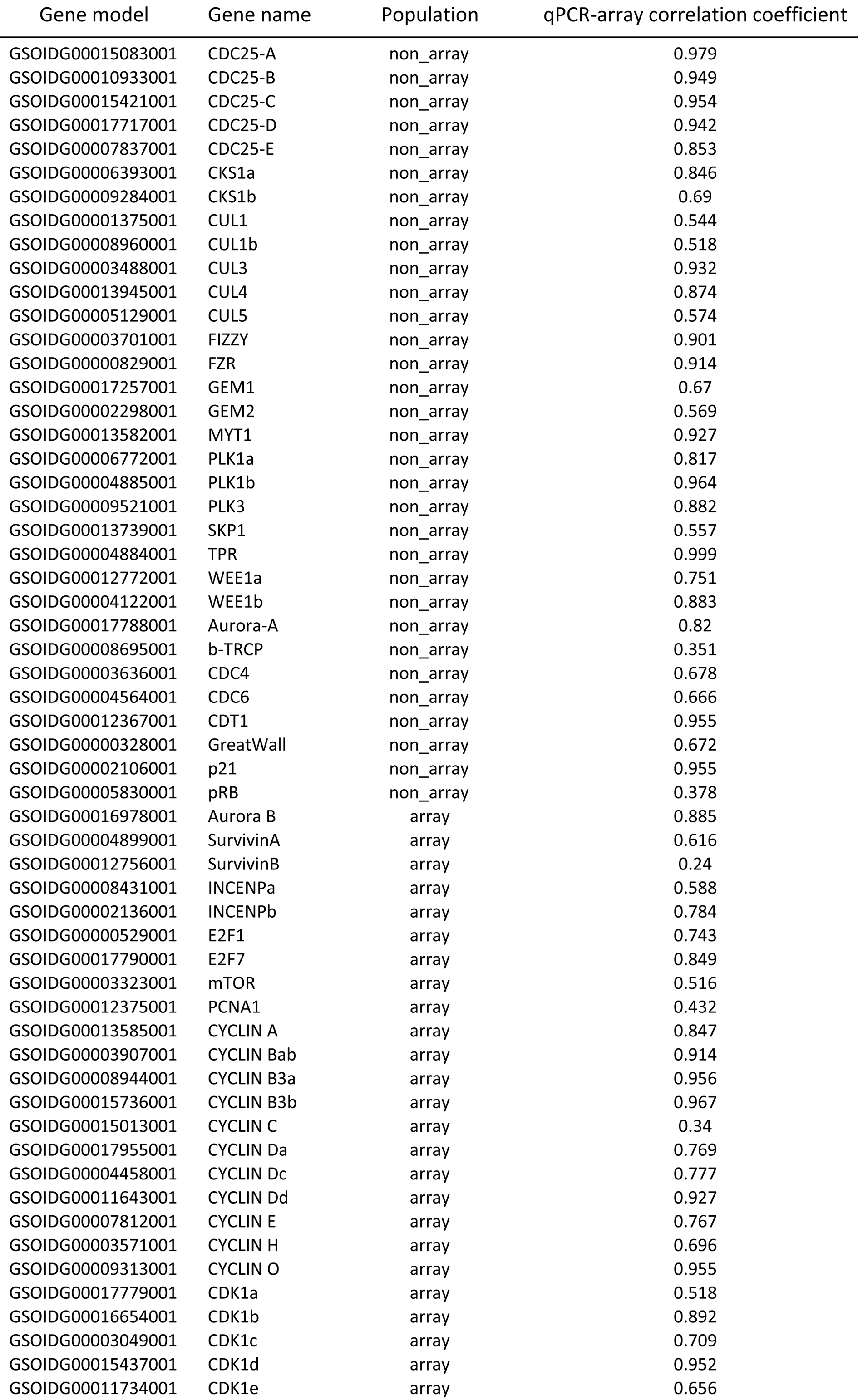
Table 1. Expression profiles of 57 genes were compared to qPCR data from 11 equivalent developmental time points using both the same population as hybridized to the tiling array (“array”) and independent populations (“non-array”). Values shown are Pearson’s correlation coefficients.
 Please Click for Larger Image
Gene ontology (GO) and InterPro domain annotation
We used Blast2GO (Götz et al., 2008) to annotate all predicted gene model protein sequences with GO terms and protein names using the nonredundant protein sequences (nr) database at an E-value cut-off of 1x10⁻³, and default weighting parameters in the GO term annotation step (see Blast2GO documentation for further details). This gave us 9667 gene models with GO annotations. We also used Blast2GO to annotate each protein with InterPro domains using InterProScan.
References
Birney,E. and Durbin, R. (2000) Using GeneWise in the Drosophila annotation experiment. Genome Res., 10, 547-548.
Bouquet,J.M., Spriet,E., Troedsson,C., Ottera,H., Chourrout,D. and Thompson,E.M. (2009). Culture optimization for the emergent zooplanktonic model organism Oikopleura dioica. J. Plankton Res., 31, 359-370.
Campsteijn,C.,Øvrebø,J.I., Karlsen,B.O. and Thompson,E.M. (2012) Expansion of cyclin D and CDK1 paralogs in Oikopleura dioica, a chordate employing diverse cell cycle variants. Mol. Biol. Evol., 29, 487-502.
Denoeud,F., Henriet,S., Mungpakdee,S., Aury,J.M., Da Silva,C., Brinkmann,H., Mikhaleva,J., Olsen,L.C., Jubin,C., Cañestro,C., et al. (2010) Plasticity of animal genome architecture unmasked by rapid evolution of a pelagic tunicate. Science., 330, 1381-1385.
Ganot,P., Kallesø,T. and Thompson,E.M. (2007) The cytoskeleton organizes germ nuclei with divergent fates and asynchronous cycles in a common cytoplasm during oogenesis in the chordate. Oikopleura. Dev. Biol., 302, 577-590.
Götz,S., Garcíí-Gómó,J.M., Terol,J., Williams,T.D., Nagaraj,S.H., Nueda,M.J.,.,Robles,M., Taló,M., Dopazo,J., Conesa,A. (2008) High-throughput functional annotation anand data mining with the Blast2GO suite. Nucleic Acids Res., 36, 3420-3435.
Howe, K.L., Chothia,T. and Durbin, R. (2002) GA ZE: a generic framework for the integration of gene-prediction data by dynamic programming. Genome Res., 12,1418-1427.
Hunter,S., Jones,P., Mitchell,A., Apweiler,R., Attwood,T.K., Bateman,A., Bernard,T,Binns,D., Bork,P., Burge,S.et.al.,(2012) InterPro in 2011: new developments in the family and domain prediction database. Nucleic Acids Res., 40, D306-D312.
Kent,W.J. (2002) BLAT--the BLAST-like alignment tool. Genome Res., 12, 656-664.
Korf,I. (2004) Gene finding in novel genomes. BMC Bioinformatics., 5, 59.
Mott, R. (1997) EST_GENOME: a program to align spliced DNA sequences to unspliced genomic DNA. Comput. Appl. Biosci., 13, 477-478.
Parra, G. Blanco, E and Guigo, R. (2000) GeneID in Drosophila. Genome Res., 10, 511-515.
Roest Crollius,H., Jaillon,O., Bernot,A., Dasilva,C., Bouneau,L., Fischer,C., Fizames,C., Wincker,P., Brottier,P., Quétier,F., et al. (2000) Estimate of human gene number provided by genome-wide analysis using Tetraodon nigroviridis DNA sequence. Nat. Genet., 25, 235-238.
Sayers,E.W., Barrett,T., Benson,D.A., Bolton,E., Bryant,S.H., Canese,K., Chetvernin,V., Church,D.M., Dicuccio,M., Federhen,S et al. (2012) Database resources of the National Center for Biotechnology Information. Nucleic Acids Res., 40, D13-D25.
Schulmeister,A., Schmid,M. and Thompson,E.M. (2007) Phosphorylation of the histone H3.3 variant in mitosis and meiosis of the urochordate Oikopleura dioica. Chrom. Res., 15, 189-201.
Slater, G.S. and Birney, E. (2005) Automated generation of heuristics for biological sequence comparison. BMC Bioinformatics., 6, 31.
Stach,S., Winter,J., Bouquet,J.-M., Chorrout,D. and Schnabel,R. (2008) Embryology of a planktonic tunicate reveals traces of sessility. Proc. Natl. Acad Sci USA., 105, 7729-7234.
The UniProt Consortium. (2012) Reorganizing the protein space at the Universal Protein Resource (UniProt). Nucleic Acids Res. 40, D71-D75.